How I Made kNN 427x Faster than torch.cdist by Handwriting CUDA Kernels
2026-06-01
Table of Contents
- Introduction
- Background Information
- The Approach: Round 1
- Measurement methodology
- Stage 0: Choosing the baseline
- Stage 1: Reducing the compute by switching to a grid-hash kNN
- Stage 2: A CUDA kernel with a register-resident top-k
- Stage 3: Coalescing - making the L1 reads contiguous
- Stages 4-5: Fold the build into the op, on-device
- Stage 6: Stop syncing with the host
- Stage 7:
float4: one 128-bit load per candidate - Stage 8: Exactness without a host sync
- Stage 9: Validation with Real Data
- End of Round 1: The kernel is at Speed of Light
- The Approach: Round 2: Pushing past the L2 wall
- The Whole Journey
- Future work and why I stopped here
Introduction
Okay, 427x faster sounds like a LOT. However, quite a few of the improvements are very specific to my use-case.
In this blog, I will describe the 12 stages of optimisations and experimentation that I went through to finish off with a hand-written, cache-resident, host-sync-free CUDA op.
The purpose of this investigation was to reduce the memory and computational cost of a key component of the hot path for model training and inference. The model at hand is a two-stage 3D point-cloud segmentation model that is used to label mesh data. Stage 1 takes an 8,000 point subsample of the mesh and coarsely labels it through a process that includes voxelisation. To score it against the ground truth we have to upsample the predictions back from 8,000 to the full mesh (~100,000 points). That upsample is a kNN lookup with k=1: for every point on the full mesh, find its closest voxel and copy that voxel's prediction. Stage 2 then uses the centroids of Stage 1's labels, takes a suitable bounding box around that label's region and then samples 8,000 points again. This zoomed in, hyperresolution point-cloud is then passed into the Stage 2 model for each label found in Stage 1, and then stitched back together, overriding Stage 1's predictions where appropriate.
This is on the hot path of both the training and validation steps.
Through this investigation process, we'll see that the naive one-liner using torch.cdist runs in 37 ms. torch.compile helps reduce that to 34 ms and is treated as the real baseline. By the end of this post, the same operation runs in 80 µs - a 427x speedup over the torch.compile-fused cdist via a single, self-contained CUDA op.
You'll see that the GPU profiler's Speed of Light (SOL) percentages gave a diagnosis and a direction on where to improve next, and that every win came from moving less data, fewer launches, or fewer syncs.
But the speedup isn't really the point of the post (... okay, a little. It's pretty neat!). The real value (in my opinion) is the journey: what insights I got at the end of each step and how that led to the next bottleneck to improve on.
The Problem
Given queries and references in , we want for each :
The starting point was to use torch's one-liner:
nn = torch.cdist(full, voxels).argmin(dim=1)   # [N]

# Alternatively, more useful if k > 1
# nn = torch.cdist(full, voxels).topk(k=1, largest=False).indices
It's important to note down our physical constraints. Firstly, the GPU is a RTX 4090 (sm_89) with CUDA 13.0 and 24 GB VRAM. The typical data being passed into this kernel is as follows:
- points in the mesh
- voxels
- (3D xyz coordinates for each point in the mesh)
float32dtype- nearest neighbours
Meshes were rescaled to [0,1]. Their data consists of:
vertices: [x, y, z]cell_ids: [vertex_index1, vertex_index2, vertex_index3] (indices of the vertices that make up each cell, also called a mesh's triangle).
Note that only the vertices themselves matter for the kNN, but the cell structure is what makes vertex indices near each other tend to be spatially near each other. We'll see how this becomes relevant in Stage 3's coalesced read.
The Data
A sanity check before benchmarking: what does actually look like across our real dataset?
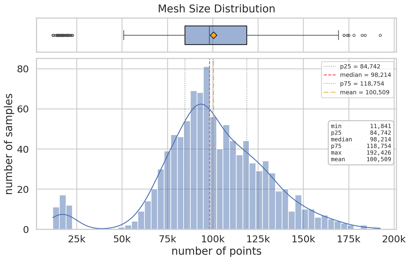
varies by ~16× across the dataset. From ~12k on small meshes to up to ~192k on dense meshes, with a median of 98,214 points. Because of this (and simplicity), I used for the optimisation process. is fixed at 8,000 regardless of mesh size, so the work scales linearly with . A small-mesh call does ~95M distance comparisons in cdist, whereas a large one does ~1.5B comparisons (~16× more for same op).
Furthering that, the meshes have different areas of local density. Their points are not uniformly distributed. This is important and highly relevant to our performance optimisations (as we'll see in Stage 9).
Realistically, we should consider the impact of the best and worst-case scenarios, especially with a quadratic compute problem, and test using a seeded sampling approach, but for this particular track, as I know the production data is more aligned to 100k +/- 20k, I just considered optimising for the median. An example of where this could go wrong is if 100k fits into L2 cache but 120k does not, for instance.
Background Information
Before jumping right in, it's worth understanding how GPU architectures work and how that ties into optimising their memory allocation.
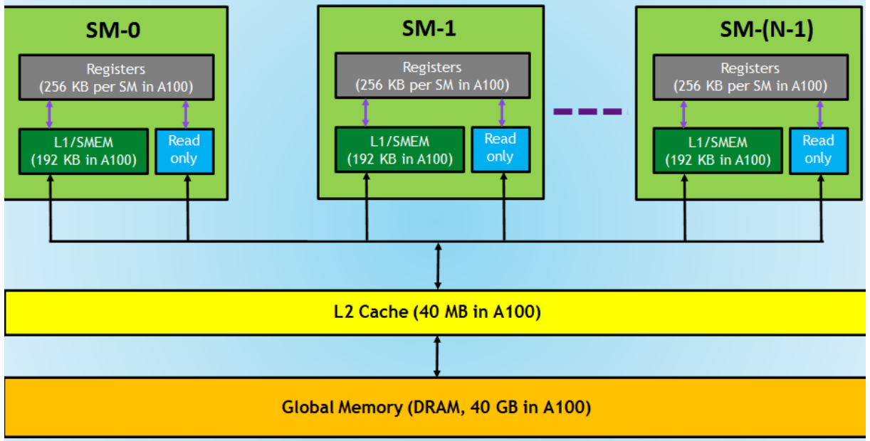
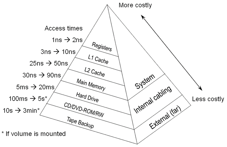
Images sourced from xoft.tistory.com/75
A modern card has dozens of Streaming Multiprocessors (SMs) - 128 on an RTX 4090. Each SM runs threads in groups of 32 (a warp) and switches between many resident warps to hide memory latency. To use the GPU well you need enough independent work to keep every SM fed, and memory access patterns that don't stall those warps waiting on data.
Each SM has its own small, fast scratch: registers (~256 KB) and a combined L1/shared memory (~128–192 KB) you control directly. All SMs share an L2 cache (72 MB on a 4090) and a much larger but much slower global DRAM (24 GB on a 4090). The latency and bandwidth gap between each tier is roughly an order of magnitude:
| Tier | Size | Latency | Scope | Bandwidth |
|---|---|---|---|---|
| Registers | 256 KB/SM | ~1 cycle (no bank conflict) | Per thread | ~3.9 TB/s/SM, ~500 TB/s aggregate (peak-issue upper bound) |
| L1 / shared mem | 128 KB/SM (split) | ~30 cycles | L1: per SM Shared: per block | ~128 B/clock/SM (multi-TB/s aggregate) |
| L2 | 72 MB | ~270–285 cycles (~107 ns) | Whole GPU | ~5 TB/s aggregate |
| Global (DRAM) | 24 GB GDDR6X | ~570 cycles | Whole GPU | 1.008 TB/s (nameplate) |
Numbers are for an RTX 4090 (sm_89). Sizes, SM count, and DRAM bandwidth from the NVIDIA Ada whitepaper and CUDA Programming Guide. L1, shared, L2, and DRAM latency/bandwidth measured in Yuan et al., arXiv:2501.12084 and Chips and Cheese's RTX 4090 microbenchmarks. NVIDIA doesn't publish register file bandwidth, so the register row is a derived upper bound from disclosed sub-partition issue rate (4 warp-insts/cycle/SM × 32 lanes × 4 B × 3 operands × 2.52 GHz boost), not a measured port bandwidth.
So optimisation is mostly about data movement, not arithmetic. Modern GPUs can do tens of TFLOPs of fp32 compute, but feeding those FLOPs from DRAM is the bottleneck for almost every real workload. The practical rules of thumb are:
- Move less data. Use the smallest dtype that preserves correctness (fp32 vs fp16 vs int8). Quantise if you can.
- Move it once. Load a tile into shared memory, reuse it across many threads, write the result back.
- Coalesce accesses. Threads in a warp should touch contiguous addresses so the hardware can satisfy them in a single transaction.
- Avoid host syncs. Every
.item(),.cpu(), or implicit.to(cpu)forces the CPU and GPU to rendezvous. One sync at the end of an op is fine but one per kernel launch destroys throughput. - Fuse kernels. Each launch costs a few µs of overhead plus a full DRAM round-trip for intermediate tensors. Fewer, fatter kernels beat many thin ones.
Importantly, every kernel is limited by one resource. The roofline model states that the attainable throughput is
where is peak memory bandwidth and is arithmetic intensity (FLOPs per byte). Low ⇒ you're on the slanted part of the roofline ⇒ bandwidth-bound. High ⇒ compute-bound.
NVIDIA's profiler (ncu) reports each kernel's Speed of Light (SOL): the percentage of its theoretical peak (calculated for compute and memory):
If memory SOL is low, you're bandwidth-bound and the fix is to move less data. If memory SOL is high but compute SOL is low, you're already memory-bound and the fix is to do more work per byte loaded.
Optimise for minimum wall-clock rather than lower utilisation % or to become DRAM-bound. This can be done by (1) doing less work (fewer bytes, fewer FLOPs, fewer launches) and (2) saturating whatever resource is binding. If one resource is pegged near 100%, then that's the bottleneck and you need to cut the work landing on it. If nothing is near 100%, the kernel is latency-, launch-, or sync-bound and adding parallelism or stripping overhead becomes more important. SOL diagnoses the bottleneck but isn't necessarily a direct measure of kernel quality.
The Approach: Round 1
Measurement methodology
To ensure the measurements are meaningful and valid, every timing in this post is the median over 200 GPU-synced calls after 8 warmup calls, on an idle GPU, as reported by ncu. The bracketed range is the [p25, p75] IQR - typically sub-percent for kernel-bound stages (pure GPU jitter), but wider on the stages where a fp32 correction branch occasionally fires (which is real variance, not noise).
The format throughout is: {median} [{p25}, {p75}] ms.
Stage 0: Choosing the baseline
torch.cdist().argmin() computes the full distance matrix (brute-force kNN) via the expansion:
then uses argmin(dim=1) to get the shortest distance's index. So there are three back-to-back kernels: a squared-norms reduction, a GEMM, and an argmin.
Result: 37.299 [37.270–37.355] ms on the representative shape (synthetic, queries-on-refs).
What ncu says: The sqrt_kernel and the GEMM stream memory at DRAM 93 % SOL. They're running the bus at 93 % of its theoretical peak. The kernels are efficient.
So why is it slow? Because the algorithm moves the wrong amount of data: distance entries through DRAM (for ). The kernels are near their roofline, but... this is for an workload.
Lesson 1: Fix the algorithm before the kernel. A kernel at 93% Speed of Light can still be the thing to delete if the algorithm itself is inefficient.
Would lowering precision work?
If cdist is bandwidth-bound, the obvious next move is to halve the bytes and double the throughput by dropping to either fp16 or bf16. The kernels do get ~2× faster... but the output is wrong.
Results for synthetic data (queries-on-refs, ):
| dtype | time (ms) | dist-agreement vs truth | net |
|---|---|---|---|
cdist fp32 | 41.643 [41.295–43.118] | 1.0000 | 1.0×; correct |
cdist fp16 | 18.890 [18.595–19.409] | 0.8990 | 2.2× faster; 10 % of NNs wrong |
cdist bf16 | 18.337 [18.147–18.666] | 0.3500 | 2.3× faster; 65 % of NNs wrong |
Why? Catastrophic cancellation in the GEMM expansion . Both squared-norm terms are , the inner product is , and the answer (a small ) sits in the low bits - exactly the bits that are thrown away first in a 16-bit dtype. bf16's 7 mantissa bits destroy the signal completely. fp16's 10 bits help on well-separated points but still mis-rank ~10% of NNs at unit-cube scale.
And the wrongness depends on the data. On real meshes (references on a 2-manifold, NN distances 10–100× smaller than the bbox), cdist bf16 dist-agreement drops to 0.2535. On tightly-clustered synthetic data, it collapses to 0.0050. The closer the neighbours, the smaller the true , and the more thoroughly low precision erases it.
The agreement column is what kills these from being a suitable baseline. A 2× speedup means nothing if the answer is wrong, so I stuck with cdist fp32.
Lesson 2: Pick the baseline by correctness rather than speed. The GEMM-expansion distance formula cancels catastrophically at low precision, and the catastrophe gets worse as the data clusters.
Free performance from torch.compile
One last thing to check before settling on a baseline: I've only run eager so far. Wrapping the cdist fp32 call in torch.compile(...) lets torch try to figure out its own fused kernel, gluing the squared-norms, the GEMM, and argmin into a tighter sequence, resulting in faster compute.
| variant | time (ms) | dist-agreement |
|---|---|---|
cdist fp32 eager | 41.30 [41.04–41.85] | 1.0000 |
cdist fp32 + torch.compile | 34.13 [33.76–34.98] | 1.0000 |
1.2× speedup without algorithm change or precision loss. The compiler collapses kernel launches, removes a materialised intermediate, and picks better fusion boundaries, all whilst producing the same bit-exact NN.
Lesson 3: Always check
torch.compile. Wrap the eager op, time it, and compare. It won't fix algorithm selection, but typically shaves 10-40% off the kernel for free (or a trade in memory usage).
The Final Baseline
From here on, the baseline is torch.compile(torch.cdist().argmin(dim=1)) with float32 data.
Stage 1: Reducing the compute by switching to a grid-hash kNN
To reduce the compute from , I wrote a pure-PyTorch implementation of the grid-hashing kNN approach. This reduces compute from quadratic scale to a linear scale.
The grid-hashing kNN buckets the references into a uniform grid, then for each query only looks at its own cell and the 26 neighbours (a block) instead of all points.
Algorithm definition
Pick the cell size so each cell holds about points (target_per_cell). With references in a bounding box of volume :
With the bounding-box origin, define the cell index of a point as
Build a hash table mapping each cell to the references it contains:
For a query , the candidate set is the union of references in its own cell and the 26 neighbouring cells:
and the nearest neighbour is taken over that set rather than all references:
Each query now examines candidates instead of , which is ~108 vs 8,000 for the given scenario.
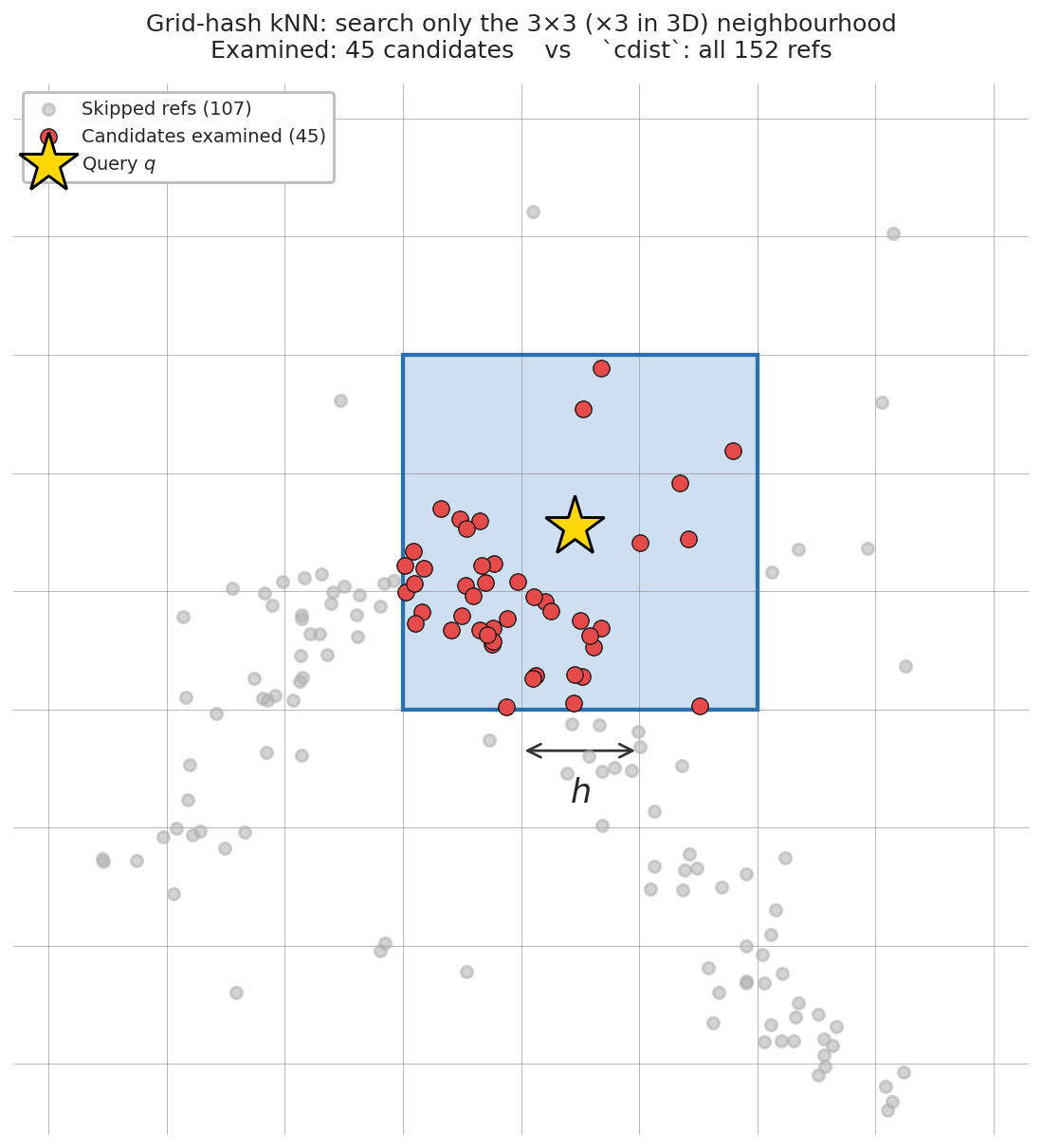
Reading the diagram: the gold star is one query . The blue-shaded cells are its 3×3 neighbourhood (this is a 2D slice for clarity, the actual algorithm uses 3×3×3 = 27 cells in 3D). The red dots are the reference points that fall inside that block, and they're the only candidates the kernel computes a distance to. The grey refs outside the block are skipped; the kernel never reads their coordinates at all.
In this toy the search shrinks ~3×. In the real workload it shrinks ~80×, to ~108 candidates per query. Neighbouring queries also share cell contents in L1/L2 cache. Together, those two effects are what eventually let us turn a DRAM-bound problem into a sub-millisecond, cache-resident kernel.
The lever here is the cell side length , sized so the average cell holds target_per_cell reference points. If is too small, the searched block contains nothing and the exactness fallback fires constantly. If is too big, the per-cell table fills up and silently truncates. Both failure modes quietly re-introduce the brute-force path we were trying to avoid.
Why it's still exact: Any reference closer than is provably inside the searched block (a point outside the block is at least away along some axis). So a query is exact whenever its k-th distance satisfies . The rare queries that violate this get an exact fallback. Concretely:
A pure-PyTorch version of this already gets ~1.8× speedup over the torch.compile-fused baseline (18.490 [18.468-18.520] ms) as it reduces the number of bytes required. As a side effect of moving less data, DRAM utilisation fell.
Accuracy Comparison of the Two Algorithms
Even though it isn't critical for my problem, torch.cdist has a real failure mode: catastrophic cancellation.
Stage 0 already showed it collapsing at low precision because of cancellation in the GEMM expansion. The cancellation doesn't actually disappear at fp32 — the arithmetic is identical, the rounding noise just shrinks to ~ instead of ~. Whether that noise mis-ranks a near-tie depends entirely on how close together those near-ties are. On well-separated data it's invisible (both methods hit 1.0000 below). On tightly-clustered data it's impactful (Stage 0's bf16 row at 0.0050 on the mesh is the same effect, just with louder noise). The grid algorithm sidesteps this entirely by construction — it never combines comparable-magnitude floats subtractively.
Grid (direct formula):
torch.cdist (GEMM expansion):
When , all three of , , are but that results in . We're subtracting two large floats whose leading bits cancel exactly. What's left is the rounding noise of , , . Each individually rounds to relative error at fp32. Cancellation can amplify that to relative error in the tiny result. A true distance of comes out as random noise, and near-ties get mis-ranked.
The direct grid formula has no cancellation step. is the genuine small difference, and subtracting two floats within a factor of 2 of each other is exact in IEEE 754, so no information is lost. Squaring a small number is fine, and summing three small non-negative squares is fine too. Nothing gets amplified anywhere.
Measured agreement vs the direct-distance truth (when , , ):
| method | dist-agreement | exactness | gap from truth |
|---|---|---|---|
torch.cdist + topk (fp32) | 1.0000 | fragile — relies on no near-ties masking the cancellation | 0 at this jitter; the cancellation collapses agreement on tightly clustered data (Stage 0's cdist bf16 table: 0.0050 on the synthetic dental arch, 0.2535 on real meshes) |
| grid-hash | 1.0000 | uses direct | 0, by construction |
At on this representative data, the jitter is large enough that the second-nearest neighbour is always well behind the first, so the GEMM cancellation has nothing to mis-rank, and both methods hit perfect exactness. But the structural difference is real, and the grid algorithm is bit-exact regardless of how clustered the data is.
Side-by-side:
cdist + topk | grid (pure PyTorch) | |
|---|---|---|
| Time complexity | , where is the average refs per cell (target_per_cell) | |
| Memory | (or chunked) | |
| Dominant cost | streaming the matrix → bandwidth-bound | candidate reads per query → cache-resident |
| Exactness | 1.0000 here; fragile to ties | 1.0000 by construction |
| Wall-clock | 34.13 ms (torch.compile-fused baseline) | 18.49 ms (1.8× over baseline) |
Stage 2: A CUDA kernel with a register-resident top-k
PyTorch still materialises the candidate gather. So I wrote a custom op that uses one thread per query, walks the 27 cells, computes distances inline, and keeps a size-k running top-k in registers. No intermediate tensor is allocated, so the only DRAM traffic is reading the inputs and writing the final indices.
Result: 83× speedup over baseline: 0.409 [0.404-0.413] ms, 100% exact. And the bandwidth profile changed completely:
| cdist | grid-hash kernel | |
|---|---|---|
| DRAM SOL | 93% | 1.4% |
| L1/TEX SOL | - | 86.9% |
The DRAM-bound problem is now cache-resident. Neighbouring queries share cells, so the candidate reads hit L1/L2 and DRAM goes quiet. The new ceiling is the L1 pipe at 87%.
Lesson 4: Re-profile after every algorithm change. When the algorithm changes, the bottleneck moves with it. We went from a DRAM wall to an L1 wall, and there would have been no way to know L1 was next without
ncu.
Stage 3: Coalescing - making the L1 reads contiguous
Why is L1 pegged? The candidate read was:
int ri = sorted_idx[p]; // p-th candidate's original index
float3 r = ((float3*)ref)[ri]; // SCATTERED — random index → fresh cache line
ri is a random original index, so each candidate touches a different cache line and the L1 pipe thrashes. To fix it, we can use the fact that mesh cells (triangles) are stored via their point indices (e.g. triangle 1 might be [0,1,2] and the connected triangle 2 might be [1,2,3]). We know they're close in space to each other, so we can pre-sort the reference coordinates into cell order. A cell's points are then contiguous in memory and a query reads them sequentially (cache-line-shared):
float3 r = ((float3*)ref_sorted)[p]; // CONTIGUOUS — coalesced, line-reused
The per-candidate sorted_idx[p] load disappears for the inner loop. We only need it to remap the winners back to original indices at the end.
Result: 99× speedup over baseline 0.344 [0.342–0.351] ms. L1/TEX SOL dropped from 86.9 % → 52.8 %, and the kernel speeds up. But now nothing is saturated (L1 ~53 %, SM ~49 %) and the kernel has become latency-bound.
Remember to measure the end-to-end call
At this point, I wanted to know why it's latency-bound, so I profiled the end-to-end call:
| Component | Share |
|---|---|
host-side grid build (torch argsort + bincount + cumsum + gather, ~15 ops) | ~60% |
| The CUDA kernel | ~32% |
| Fallback check | ~8% |
The build dominated, and it was ~15 separate PyTorch operations - each launching a tiny kernel. The GPU did a microsecond of work, then sat idle ~5–10 µs while the CPU launched the next one. So it was launch/latency-bound. No resource was near 100% utilisation and the GPU was just waiting around.
Lesson 5: Profile the whole call, not just the kernel. Amdahl's Law applies. Making the kernel faster isn't worth the time if the kernel is only 32% of wall-clock.
Stages 4-5: Fold the build into the op, on-device
So the next thing to attack was the launch count. I rebuilt the grid on the device in a single atomic kernel: one thread per reference computes its cell (matching the kernel's linearisation):
and atomicAdds itself into that cell's table. There was no more argsort or ~15 launches - just ~2 device kernels. I went further by storing the coordinates in the table so the query reads them contiguously and the build stays on-device. Both were wins, and kept it in the one op.
Stage 4 result (just the on-device atomic build, query still scattered): 0.295 [0.294–0.296] ms; 116× over baseline. Faster than the previous coalesced version, even though the query kernel itself got worse. Killing the build launches saved more time than the query lost.
Stage 5 result (build and coord-table query, both wins): 0.222 [0.221–0.223] ms; 154× over baseline.
Lesson 6: When a fix isn't impacting SOL %, look at launches or syncs.
At this point, killing the launches mattered more than any kernel tweak.
Stage 6: Stop syncing with the host
With the build gone, the next ~21% was GPU→CPU syncs in the Python wrapper. Extracting grid parameters did roughly seven separate float() / int() calls. Each one is a cudaDeviceSynchronize in disguise, stalling the pipeline ~5–20 µs:
h = float((c * extent.prod() / N) ** (1/3)) # sync
g0 = int(G[0]); g1 = int(G[1]); g2 = int(G[2]) # 3 syncs
ox = float(rmin[0]); ... # 3 syncs
Collapse them into one host transfer:
ex0, ex1, ex2 = extent.tolist() # ONE sync; derive h, inv_h, g0..g2 on the CPU
ox, oy, oz = rmin.tolist() # ONE sync
Seven syncs became two, reducing host-overhead.
Result: 0.171 [0.171–0.172] ms - a 200× speedup over baseline. This was the single biggest lever after folding the build on-device, which confirms the op was sync/host-bound, not kernel-bound, at this data size.
Lesson 7: Once the kernel is fast enough, host syncs and launch overhead become the bottleneck.
Stage 7: float4: one 128-bit load per candidate
L1 was once again the bottleneck (the candidate-coord loads saturate the load-store unit). A float3 is 12 bytes, which isn't a native vector width, so it compiles to two loads. So I packed the coordinate and the original index into a 16-byte, 16-byte-aligned float4:
// build: one slot = (x, y, z, idx-as-float-bits)
table4[slot] = make_float4(rx, ry, rz, __int_as_float(i));

// query: ONE LDG.128 carries coord AND index
float4 r = table4[base + t];
float d2 = (qx-r.x)*(qx-r.x) + (qy-r.y)*(qy-r.y) + (qz-r.z)*(qz-r.z);

// winner index comes straight from r.w - no separate index table or remap
One wide aligned load replaces two narrow ones, and the separate index table and end-of-loop remap vanish. The query kernel cost went from 140 µs → 90 µs; L1/TEX 84.7% → 52.3%, and the bottleneck moved to L2 (~79%).
Stage 8: Exactness without a host sync
One sync remained: deciding whether to run the exact fallback required reading a GPU boolean to the host (uncertain.any()). So I replaced the whole Python fallback with a branchless GPU correction kernel baked into the op:
// h² is recoverable from inv_h - no new argument
if (out_d2[j*k + (k-1)] <= h2) continue; // already exact: one read + continue
// else: brute-force this query's top-k over all refs, overwrite. No host sync.
The common case (in the real workload, every query) is a single read-and-continue. I also closed a latent correctness gap: dense cells that overflow the fixed table get truncated, so a query could look exact yet miss the true NN. The query kernel now flags overflow and poisons that query's distance to to force the correction. This makes it exact even under truncation.
The op is now fully self-contained into three device kernels: build → query → correct, and the Python side does nothing but compute params and cast a dtype. No host syncs remained in the call.
Result: 0.109 [0.108–0.110] ms - 313× over baseline.
The IQR collapses to sub-percent here. That's Round 1 done structurally: the op is fully self-contained, no host syncs remain in the call, and we're now bandwidth-bound on L2.
Stage 9: Validation with Real Data
Awkward realisation: I'd been benchmarking on uniform-random queries and references, drawn independently. On that data, lots of queries land far from any reference, so their k-th distance exceeds and the exact fallback fires on most of them, which dominates the time.
But real meshes are the exact opposite: every query sits essentially on a voxel, so and the fallback never fires. Re-benchmarking on representative data (query = voxel + small jitter):
| variant | uniform "stress" | representative (real use) |
|---|---|---|
| cdist | 37.30 [37.27–37.36] ms | 37.30 [37.27–37.36] ms |
| grid kernel (coalesced) | 0.346 [0.342–0.351] ms | 0.344 [0.342–0.351] ms |
| final op | 0.084 [0.084–0.085] ms | 0.080 [0.079–0.081] ms |
Lesson 8: Benchmark the distribution you actually run. Synthetic data that doesn't match production will point you at bottlenecks that might be of a different data distribution.
End of Round 1: The kernel is at Speed of Light
Final round-1 query kernel, ncu Speed-Of-Light section, representative data (87 µs kernel, 0.109 ms end-to-end):
| SOL metric | value |
|---|---|
| Memory Throughput | 81.0% |
| L2 Cache Throughput | 81.0% |
| L1/TEX Cache Throughput | 59.7% |
| DRAM Throughput | 4.1% |
| Compute (SM) Throughput | 28.4% |
ncu's own verdict:
"This workload is utilizing greater than 80.0% of the available compute or memory performance of the device. Start by analyzing L2."
The kernel is at 81% of its memory Speed of Light, gated by L2 cache throughput. It's streaming the cache-resident candidate table about as fast as L2 can serve it. Compute, meanwhile, is sitting idle at 28%. The actual arithmetic is tiny (~ MFLOP, under 1% of the 4090's ~80 TFLOP/s), so we're definitively bandwidth-bound. There's no arithmetic lever left.
That sets up Round 2: instead of going faster, the goal is to push fewer bytes through L2.
The Approach: Round 2: Pushing past the L2 wall
Stage 9: Fusing the query and correction kernels
Round 1 had two device kernels in the call: query, then correction. We can fuse them by adding the per-thread correction as a single branch at the end of the query loop. This results in no out_d2 round-trip and one fewer launch.
Result: 0.106 [0.106–0.107] ms; 322× speedup over baseline. Marginal end-to-end, just saving on launch overhead (~3 µs), but every µs counts at this point.
Stage 10: Halving the bytes
Each candidate read was 16 bytes (a float4). Storing it as fp16 would halve the L2 traffic for the same work. But which 16-bit format?
| exponent | mantissa | relative precision | range | |
|---|---|---|---|---|
| fp16 | 5 | 10 | ±65504 | |
| bf16 | 8 | 7 | ±3×10³⁸ |
A coordinate's quantisation error is . Our coordinates are bounded (a point cloud in a small box), so bf16's enormous range is wasted. What matters for ranking near neighbours is precision, and fp16 has ~8× more of it. So fp16 is the better option over bf16.
We store coordinates origin-relative (small magnitudes avoid cancellation in ), pack them into an 8-byte half4 (one LDG.64), and keep the integer index in a parallel table read only for the winners. The fp32 brute-force correction stays the exactness backstop for any fp16 near-tie.
Result: 0.097 [0.097–0.098] ms - 352× speedup over baseline. This wasn't as big of an improvement as halving the bytes might suggest, because on real data the home cell already holds the nearest voxel, so we weren't reading many candidate bytes to begin with. Time to focus on cutting work, not bytes.
Stage 11: Early termination to avoid redundant compute
Up until now, we'd been searching all 27 cells to guarantee correctness. But for k=1, once you've found a close enough candidate, a far cell can't possibly contain anything nearer. So we should skip the cell whenever the minimum possible distance from the query to that cell's box already loses:
On real data the home cell (the one containing ) sets tiny, and most of the other 26 cells get pruned before a single byte is read.
Result: 0.080 [0.079–0.081] ms - 427× over baseline. The profile confirms we reduced the demand on L2: L2 SOL 81 % → 72.6 %, kernel 87 µs → 52 µs.
Stage 12: Collapse the host overhead
With the kernel now roughly 40% smaller, the fixed overhead suddenly looked like a big portion of the op. We'd already fused the query and correction kernels into one, so the remaining job was to collapse the grid parameters into a single host sync — replacing the separate float() / int() calls with torch.cat([rmin, extent]).tolist(), a single transfer for everything.
Result: 0.080 [0.079–0.081] ms - 427× over baseline with just one host sync. At the kernel work has already shrunk below the host overhead Stage 11 was paying, so this collapse just removes a remaining overhead source without adding a measurable wall-clock win on top of Stage 11. At larger (I measured ~0.009 ms of headroom at ) it does pay off. So Stage 12 starts mattering once gets bigger than 100k; at 100k itself, Stage 11 and Stage 12 share the floor.
The Whole Journey
Representative shape (queries-on-refs + small jitter, , , , , RTX 4090, median of 200 calls).
| stage | what changed | bottleneck after | time (ms) | vs baseline |
|---|---|---|---|---|
| 0 | torch.cdist (eager fp32) | DRAM 93 % (O(N²) bytes) | 37.299 [37.270–37.355] | 0.92× |
| 0b | cdist fp32 + torch.compile | baseline | 34.133 [33.758–34.977] | 1.0× |
| 1 | spatial grid (pure PyTorch) | torch dispatch | 18.490 [18.468–18.520] | 1.8× |
| 2 | CUDA register top-k | L1 87 % | 0.409 [0.404–0.413] | 83× |
| 3 | coalesced (cell-sorted) | L1 53 %, nothing saturated | 0.344 [0.342–0.351] | 99× |
| 4 | build folded on-device (atomic) | scattered query gather | 0.295 [0.294–0.296] | 116× |
| 5 | + coord table (coalesced query) | L1/tex 85 % | 0.222 [0.221–0.223] | 154× |
| 6 | batch host syncs (7 → 2) | kernel ~32 % of op | 0.171 [0.171–0.172] | 200× |
| 7 | float4 packed load (LDG.128) | L1 52 %, L2 79 % | 0.130 [0.129–0.130] | 263× |
| 8 | GPU exact-correction, no host sync | L2 81 % (SOL) | 0.109 [0.108–0.110] | 313× |
| 9 | fuse query + correction kernels | one fewer launch | 0.106 [0.106–0.107] | 322× |
| 10 | fp16 coord table (half4, LDG.64) | fewer bytes / candidate | 0.097 [0.097–0.098] | 352× |
| 11 | early termination (cell pruning) | L2 72.6 %, kernel 87 → 52 µs | 0.080 [0.079–0.081] | 427× |
| 12 | one host sync | kernel-floor reached at this | 0.080 [0.079–0.081] | 427× |
The op became 427× faster than the post-compiled baseline (≈466× over the eager-cdist one-liner), fully exact, one host sync, in a single self-contained CUDA op.
The Lessons (in one place)
- Fix the algorithm before the kernel. A kernel at 93% SOL can still be the wrong algorithm.
- Pick the baseline by correctness rather than speed.
- Always check what
torch.compilecan find for free, and make it your baseline. - Re-profile after every algorithm change. When the algorithm changes, so does the bottleneck.
- Profile the whole call, not just the kernel. Amdahl's Law applies: the kernel here was only 32%; the build was 60%.
- When a fix isn't moving a SOL %, look at launches or syncs. ~15 tiny ops are mostly idle gaps. Fuse and batch where possible.
- Once the kernel is fast enough, host syncs and launch overhead become the bottleneck.
- Benchmark the distribution you actually run. Synthetic data that doesn't match production points you at bottlenecks that aren't there.
- Report uncertainty. Median-only timing hides whether a 10% "win" is signal or noise. Sub-percent IQRs on kernel-bound stages confirm the improvement is real.
Future work and why I stopped here
I stopped at 0.080 [0.079–0.081] ms (427× over the torch.compile-fused baseline) because the remaining levers all have steeply diminishing returns on a sub-0.1 ms primitive. The kernel is near its memory roofline and the remaining ~45% is host overhead, which would need CUDA graphs to seriously dent.
For completeness, here are the TODOs I considered and parked:
- CUDA graph the GPU portion: After round 2 the op is only ~55% kernel. The other ~45% is host overhead: parameter computation, one sync, two kernel launches, a
memset. Capturing the GPU work (memset + build + fused-query) into a CUDA graph and replaying it amortises the launch overhead to near zero across repeated calls. It's the one lever still aimed at the actual bottleneck (overhead), but it'd probably result in an improvement of ~10% of a 0.080 ms op and adds graph-capture machinery and shape-bucketing complexity. - Block-cooperative shared memory: Staging each cell's points into shared memory once and reusing them across a thread block is the best way to beat an L2-bandwidth ceiling. But two things killed its ROI: after fp16 + early termination the kernel is no longer L2-saturated (72%, drifting latency-bound), and it's only ~55% of the op. It also needs the queries sorted by cell so a block shares cells. A perfect SMEM kernel would save maybe <15 µs of the 80 µs. This is high effort as it requires a query-sort rewrite.
- Larger
kand approximate modes. Everything here is tuned for exactk=1(the voxel→full case). The register top-k caps neark≈32; beyond that,torch.topk's radix-select wins. An approximate mode would shave the correction check, but exactness helped for my use-case.
Final tally: cdist fp32 + torch.compile at 34.13 [33.76–34.98] ms → grid op at 0.080 [0.079–0.081] ms = 427×, with one host sync, in a single self-contained CUDA op.
End to end, this optimisation journey freed up a chunk of memory and saved around 10–15% wall-clock during training overall.